amep.evaluate.PCFangle#

class amep.evaluate.PCFangle(traj: ParticleTrajectory, skip: float = 0.0, nav: int = 10, ptype: int | None = None, other: int | None = None, mode: str = 'psi6', max_workers: int | None = 1, **kwargs)#

Bases: BaseEvaluation

2d angular pair correlation function.

__init__(traj: ParticleTrajectory, skip: float = 0.0, nav: int = 10, ptype: int | None = None, other: int | None = None, mode: str = 'psi6', max_workers: int | None = 1, **kwargs) → None#

Calculate the two-dimensional pair correlation function \(g(r,\theta)\).

Implemented for a 2D system. Takes the time average over several time steps.

Three modes are available, the default, 'psi6' allows for averaging the result (either with respect to time or to make an ensemble average), the coordinates are rotated such that the mean \(\psi_6\) orientation points along the \(x\)-axis (see Ref. [1] for details).

The mode 'orientations' calculates \(g(r,\theta)\) in relation to the individual particle orientations (frame.orientations()). This mode is particularly interesting for active matter.

The mode 'x' calculates \(g(r,\theta)\) in relation to the \(x\)-axis.

Per default, it is assumed that the system has periodic boundary conditions (keyword pbc=True). Please adjust as needed. The keyword pbc is forwarded to amep.spatialcor.pcf_angle() via **kwargs.

Notes

The angle-dependent pair correlation function is defined by (see Ref. [2])

\[g(r,\theta) = \frac{1}{\langle \rho\rangle_{\text{local},\theta} N}\sum\limits_{i=1}^{N} \sum\limits_{j\neq i}^{N}\frac{\delta(r_{ij} -r)\delta(\theta_{ij}-\theta)}{2\pi r^2 \sin(\theta)}\]

The angle \(\theta\) is defined with respect to a certain axis \(\vec{e}\) and is given by

\[\cos(\theta)=\frac{\vec{r}_{ij}\cdot\vec{e}}{r_{ij}e}\]

The vector \(\vec{e}\) is default the x-axis, but can be specified by supplying the parameter e. See parameter description for details.

The angles are in the range \(\theta \in [0, 2\pi)\).

This method only works for 2D systems.

References

Parameters:

traj (ParticleTrajectory) – Trajectory object with particle-based simulation data.
skip (float, optional) – Skip this fraction at the beginning of the trajectory. The default is 0.0.
nav (int, optional) – Number of frames to consider for the time average. The default is 10.
ptype (int or None, optional) – Particle type. The default is None.
other (int or None, optional) – Other particle type (to calculate the correlation between different particle types). other will specify the locations of the reference particles from which the distances and angles to the particles ptype are calculated (”other ≙ probing locations”). The default is None which uses the ptype particles.
mode (str, optional) – Mode that defines with respect to which axis the angles are calculated. Possible values are 'psi6', 'orientations', and 'x'. The default is 'psi6', which uses the hexagonal order parameter to define the mean orientation. The option orientations calculates \(g(r,\theta)\) with respect to the individual particle orientations (useful for active particles). The option 'x' uses the \(x\)-axis of the simulation box as reference. The default is 'psi6'. different particle types). The default is None.
max_workers (int or None, optional) – Number of parallel workers. Will be forwarded to utils.average_func.
**kwargs – All other keyword arguments are forwarded to amep.spatialcor.pcf_angle().

Examples

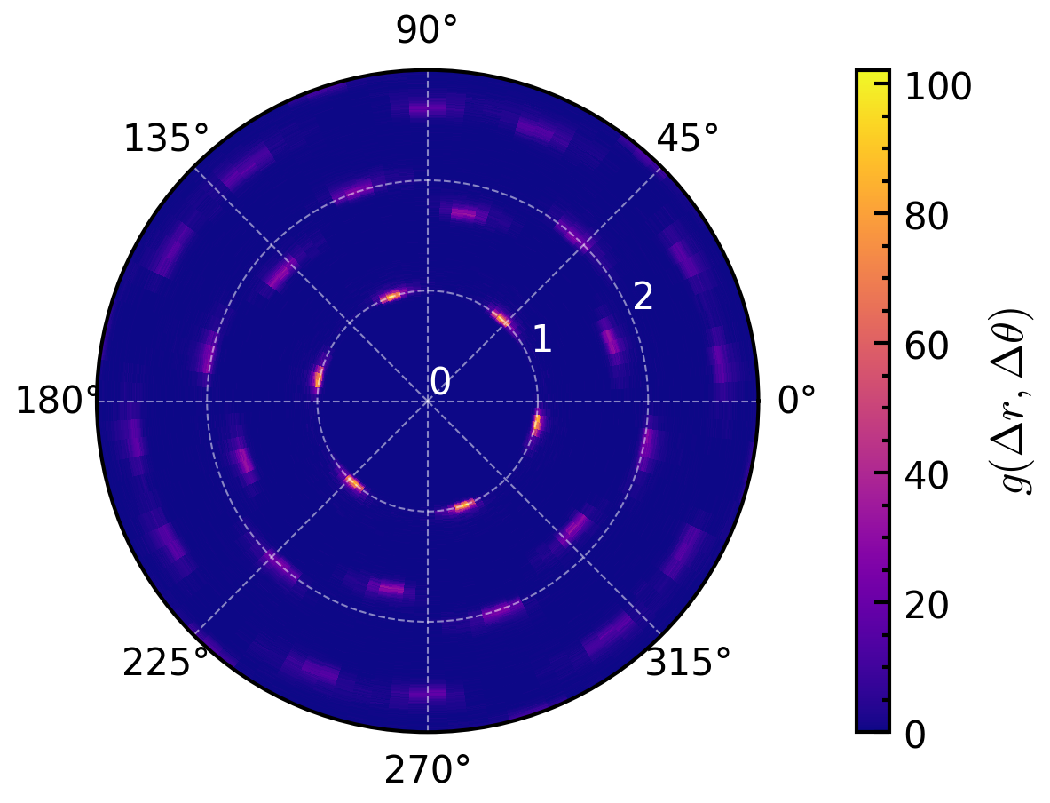
>>> import amep
>>> traj = amep.load.traj("../examples/data/lammps.h5amep")
>>> pcfangle = amep.evaluate.PCFangle(traj, skip=.9, nav=2, rmax=3)
>>> fig, axs = amep.plot.new(subplot_kw=dict(projection="polar"))
>>> mp = axs.pcolormesh(pcfangle.theta, pcfangle.r, pcfangle.avg)
>>> cax = amep.plot.add_colorbar(fig, axs, mp, label=r"$g(\Delta r, \Delta \theta)$")
>>> axs.grid(alpha=.5, lw=.5, c='w')
>>> axs.set_rticks([0,1,2,3])
>>> axs.tick_params(axis='y', colors='white')
>>>
>>> fig.savefig("PCFangle_1.png")

>>>
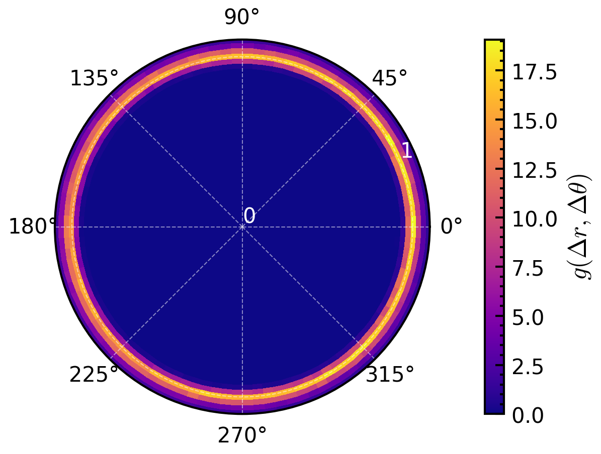
>>> # PCFangle in relation to the particle orientations
>>> pcfangle = amep.evaluate.PCFangle(traj, skip=.75,
>>>                 nav=10, rmax=3, nabins=100,
>>>                 ndbins=100, mode="orientations"
>>>                 )
>>> fig, axs = amep.plot.new(subplot_kw=dict(projection="polar"))
>>> mp = axs.pcolormesh(pcfangle.theta, pcfangle.r, pcfangle.avg)
>>> cax = amep.plot.add_colorbar(fig, axs, mp, label=r"$g(\Delta r, \Delta \theta)$")
>>> axs.grid(alpha=.5, lw=.5, c='w')
>>> axs.set_rticks([0,1,2,3])
>>> axs.set_rlim(0,1.1)
>>> axs.tick_params(axis='y', colors='white')
>>>
>>> fig.savefig("PCFangle_2.png")

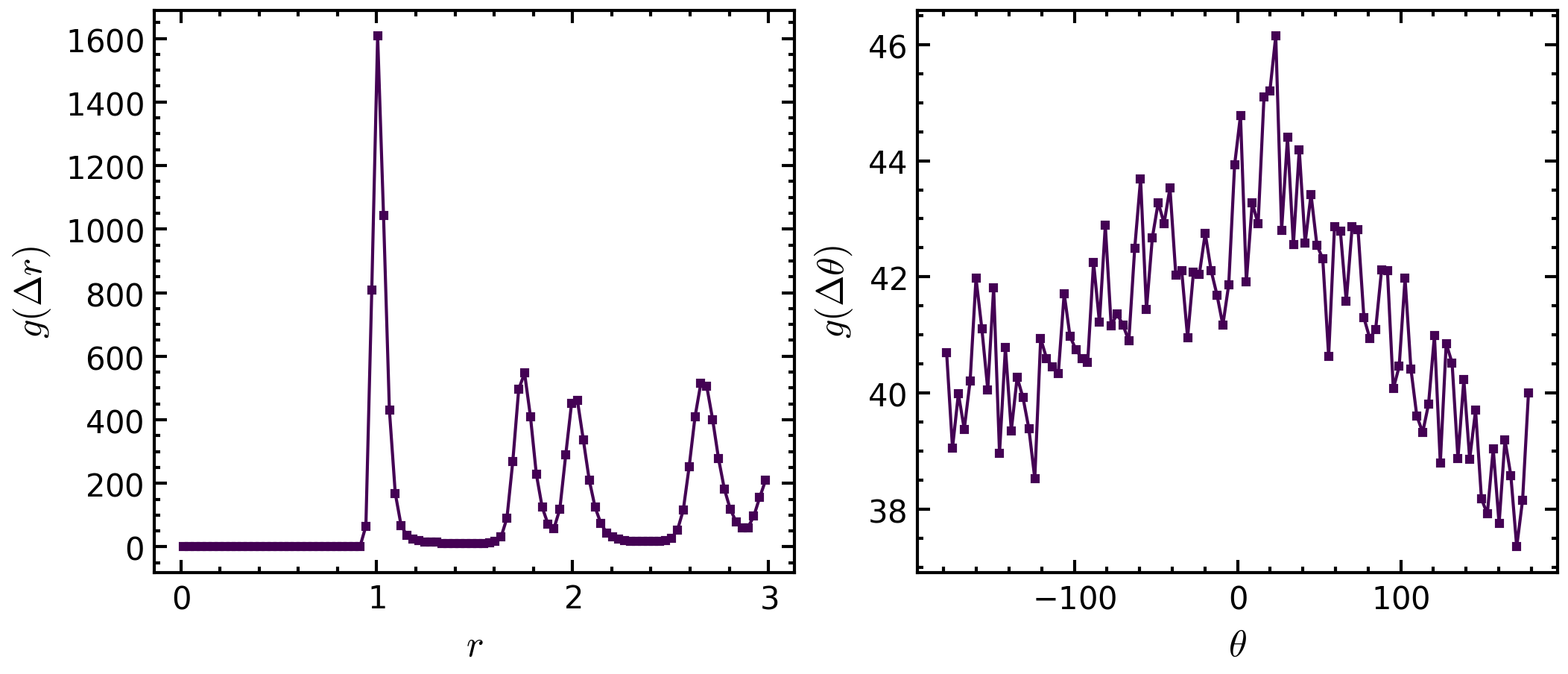
>>> # plot integrated histograms to have 1d-plots
>>> fig, axs = amep.plot.new((7,3), ncols=2)
>>> angles = pcfangle.theta[:,0]
>>> theta_integrated = np.sum(pcfangle.avg, axis=0)
>>> axs[0].plot(np.mean(pcfangle.r, axis=0), theta_integrated)
>>> axs[0].set_xlabel(r"$r$")
>>> axs[0].set_ylabel(r"$g(\Delta r)$")
>>>
>>> # fig, axs = amep.plot.new()
>>> # only integrate over first peak
>>> r_integrated = np.sum(pcfangle.avg*(pcfangle.r<1.1), axis=1)
>>> # changing angles so that it is plottet around 0
>>> theta=np.mean(pcfangle.theta, axis=1)
>>> angles=(angles+np.pi)%(2*np.pi)-np.pi
>>> angles*=180/np.pi # to change from radians to degree
>>> # sorting so that data points are plotted in order
>>> sort=np.argsort(angles)
>>> axs[1].plot(angles[sort], r_integrated[sort])
>>> axs[1].set_xlabel(r"$\theta$")
>>> axs[1].set_ylabel(r"$g(\Delta \theta)$")
>>>
>>> fig.savefig("PCFangle_3.png")

Methods

`__init__`(traj[, skip, nav, ptype, other, ...])	Calculate the two-dimensional pair correlation function \(g(r,\theta)\).
`items`()
`keys`()	The keys to the evaluation object.
`save`(path[, backup, database, name])	Stores the evaluation result in an HDF5 file.
`values`()

Attributes

`avg`	Time-averaged PCFangle (averaged over the given number of frames).
`frames`	PCFangle for each frame.
`indices`	Indices of all frames for which the PCFangle has been evaluated.
`name`
`r`	Distances.
`theta`	Angles.
`times`	Times at which the PCFangle is evaluated.

property avg#

Time-averaged PCFangle (averaged over the given number of frames).

Returns:: Time-averaged function value.
Return type:: np.ndarray

property frames#

PCFangle for each frame.

Returns:: PCFangle for each frame.
Return type:: np.ndarray

property indices#

Indices of all frames for which the PCFangle has been evaluated.

Returns:: Frame indices.
Return type:: np.ndarray

keys() → list[str]#

The keys to the evaluation object.

Used so Evaluation-objects can be used as dictionaries.

property r#

Distances.

Returns:: Distances.
Return type:: np.ndarray

save(path: str, backup: bool = True, database: bool = False, name: str | None = None) → None#

Stores the evaluation result in an HDF5 file.

Parameters:

path (str) – Path of the ‘.h5’ file in which the data should be stored. If only a directory is given, the filename is chosen as self.name. Raises an error if the given directory does not exist or if the file extension is not ‘.h5’.
backup (bool, optional) – If True, an already existing file is backed up and not overwritten. This keyword is ignored if database=True. The default is True.
database (bool, optional) – If True, the results are appended to the given ‘.h5’ file if it already exists. If False, a new file is created and the old is backed up. If False and the given ‘.h5’ file contains multiple evaluation results, an error is raised. In this case, database has to be set to True. The default is False.
name (str or None, optional) – Name under which the data should be stored in the HDF5 file. If None, self.name is used. The default is None.

Return type:

None.

property theta#

Angles.

Returns:: Angles.
Return type:: np.ndarray

property times#

Times at which the PCFangle is evaluated.

Returns:: Times at which the PCFangle is evaluated.
Return type:: np.ndarray

amep.evaluate.PCFangle#

This Page