amep.functions.MaxwellBoltzmann#
- class amep.functions.MaxwellBoltzmann(d: int = 1, m: float = 1.0)#
Bases:
BaseFunctionMaxwell-Boltzmann distribution.
- __init__(d: int = 1, m: float = 1.0)#
Maxwell-Boltzmann velocity distribution.
Initializes a function object of a Maxwell-Boltzmann distribution. This distribution describes velocities of free particles in thermal equilibrium. It is usually derived in three dimensions where it is
\[f(v) = {\left[\frac{m}{2\pi{}k_bT}\right]}^\frac{3}{2}4\pi{} v^2\exp\left(-\frac{mv^2}{k_bT}\right)\]in arbitrary spatial dimensions \(d\) it is given by
\[f(v) = \frac{2}{\Gamma\left(\frac{d}{2}\right)} {\left[\frac{m}{k_bT}\right]}^\frac{d}{2} v^{d-1}\exp\left(-\frac{mv^2}{k_bT}\right)\]- Parameters:
d (int, optional) – Spatial dimension. The default is 1.
m (float, optional) – Mass (if None, set to unity). The default is None.
- Return type:
None.
Examples
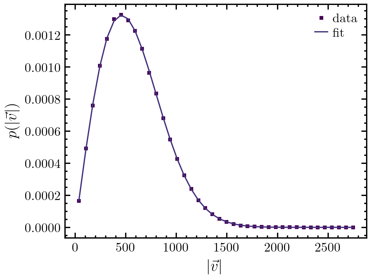
>>> import amep
>>> traj = amep.load.traj("../examples/data/lammps.h5amep")
>>> vdist = amep.evaluate.VelDist(traj, skip=0.0, nav=100)
>>> vfit = amep.functions.MaxwellBoltzmann(d=2, m=1.0)
>>> vfit.fit(vdist.v, vdist.vdist, p0=[1000.0])
>>> fig, axs = amep.plot.new()
>>> axs.plot(
...     vdist.v, vdist.vdist, label='data', ls=""
... )
>>> axs.plot(
...     vdist.v, vfit.generate(vdist.v),
...     marker="", label='fit'
... )
>>> axs.legend()
>>> axs.set_xlabel(r'$|\vec{v}|$')
>>> axs.set_ylabel(r'$p(|\vec{v}|)$')
>>> fig.savefig('./figures/functions/functions-MaxwellBoltzmann.png')
Methods
__init__([d, m])Maxwell-Boltzmann velocity distribution.
f(p, x)Calculate the value of the Maxwell-Boltzmann distribution.
fit(xdata, ydata[, p0, sigma, maxit, verbose])Fits the function self.f to the given data by using ODR (orthogonal distance regression).
generate(x[, p])Returns the y values for given x values.
Attributes
Returns the fit errors for each parameter as an array.
keysmeannamenparamsoutputReturns an array of the optimal fit parameters.
Returns the dictionary of fit results including parameter names, parameter values, and fit errors.
std- property errors: ndarray#
Returns the fit errors for each parameter as an array.
- Returns:
Fit errors.
- Return type:
np.ndarray
- f(p: list[float] | ndarray, x: float | ndarray) float | ndarray#
Calculate the value of the Maxwell-Boltzmann distribution.
This distribution describes velocities of free particles in thermal equilibrium. It is usually derived in three dimensions where it is
\[f(v) = {\left[\frac{m}{2\pi{}k_bT}\right]}^\frac{3}{2}4\pi{} v^2\exp\left(-\frac{mv^2}{k_bT}\right)\]in arbitrary spatial dimensions \(d\) it is given by
\[f(v) = \frac{2}{\Gamma\left(\frac{d}{2}\right)} {\left[\frac{m}{k_bT}\right]}^\frac{d}{2} v^{d-1}\exp\left(-\frac{mv^2}{k_bT}\right)\]- Parameters:
p (list | np.ndarray) – Parameters \(k_{\rm B}T\).
x (float | np.ndarray) – Velocities(s) \(v\) at which the function is evaluated.
- fit(xdata: ndarray, ydata: ndarray, p0: list | None = None, sigma: ndarray | None = None, maxit: int | None = None, verbose: bool = False) None#
Fits the function self.f to the given data by using ODR (orthogonal distance regression).
- Parameters:
xdata (np.ndarray) – x values.
ydata (np.ndarray) – y values.
p0 (list or None, optional) – List of initial values. The default is None.
sigma (np.ndarray or None, optional) – Absolute error for each data point. The default is None.
maxit (int, optional) – Maximum number of iterations. The default is 200.
verbose (bool, optional) – If True, the main results are printed. The default is False.
- Return type:
None.
- generate(x: ndarray, p: list | None = None) ndarray#
Returns the y values for given x values.
- Parameters:
x (np.ndarray) – x values.
p (list, optional) – List of parameters. The default is None.
- Returns:
y – f(x)
- Return type:
np.ndarray
- property params: ndarray#
Returns an array of the optimal fit parameters.
- Returns:
Fit parameter values.
- Return type:
np.ndarray
- property results: dict#
Returns the dictionary of fit results including parameter names, parameter values, and fit errors.
- Returns:
Fit results.
- Return type:
dict