amep.functions.gaussian2d

amep.functions.gaussian2d(data_tuple: tuple[ndarray, ndarray], A: float, mux: float, muy: float, sigx: float, sigy: float, theta: float, offset: float) → ndarray

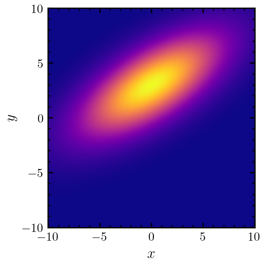
2D Gaussian Bell curve.

Equivalent to the probability density function of a normal distribution in two dimensions. By the central limit theorem this is a good guess for most peak shapes that arise from many random processes. This parametrization can include correlations via the angle variable \(\theta\). The function is given by

\[g(x)= A\exp\left(-\left(\vec{x}-\vec{\mu}\right)^T R(\Theta)^{-1}\sigma^{-2}R(\Theta) \left(\vec{x}-\vec{\mu}\right) \right)+b\]

where \(\vec{x}\) is the vector composed the x and y coordinates, \(\vec{\mu}\) is the mean vector composed of \(\mu_x\) and \(\mu_y\) and \(\sigma^{-2}\) is the diagonal matrix with the inverse variances \(\sigma_x^{-2}\) and \(\sigma_y^{-2}\) as entries.

Parameters:

• data (tuple) – tuple (x,y) of x and y values where x and y are 1D np.ndarrays.

• A (float) – amplitude.

• mux (float) – mean \(\mu_x\) in x direction.

• muy (float) – mean \(\mu_y\) in y direction.

• sigx (float) – standard deviation \(\sigma_x\) in x direction.

• sigy (float) – standard deviation \(\sigma_y\) in y direction.

• theta (float) – Orientation angle \(\Theta\) of the polar axis.

• offset (float) – offset \(b\). Shifts the output value linearly.

Returns:

g(x) – 1D array of floats (flattended 2D array!)

Return type:

np.ndarray

Examples

>>> import amep
>>> import numpy as np
>>> x = np.linspace(-10, 10, 500)
>>> y = np.linspace(-10, 10, 500)
>>> X,Y = np.meshgrid(x,y)
>>> z = amep.functions.gaussian2d(
...     (X,Y), 1.0, 0.0, 3.0, 2.0, 5.0, np.pi/3, 0.0
... ).reshape((len(x),len(y)))
>>> fig, axs = amep.plot.new(figsize=(3,3))
>>> amep.plot.field(axs, z, X, Y)
>>> axs.set_xlabel(r'$x$')
>>> axs.set_ylabel(r'$y$')
>>> fig.savefig('./figures/functions/functions-gaussian2d-function.png')