amep.spatialcor.pcf_angle

amep.spatialcor.pcf_angle(coords: ndarray, box_boundary: ndarray, other_coords: ndarray | None = None, ndbins: int = 500, nabins: int = 100, rmax: float | None = None, psi: ndarray | None = None, njobs: int = 1, pbc: bool = True, verbose: bool = False, chunksize: int | None = None, e: ndarray = array([1., 0., 0.])) → tuple[ndarray, ndarray, ndarray]

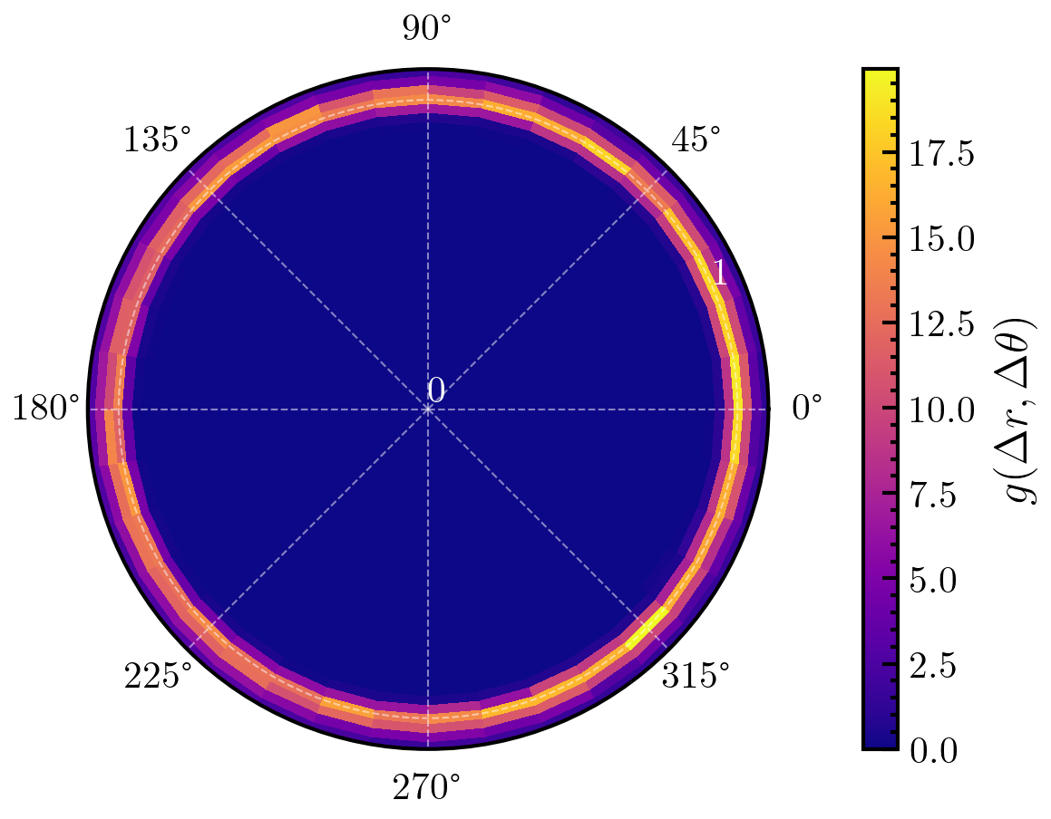
Calculate the angle dependent radial pair correlation function.

Do that by calculating histograms. To allow for averaging the result (either with respect to time or to make an ensemble average), the coordinates are rotated such that the mean orientation (given by the vector psi) points along the x axis (see Ref. [1] for details).

Notes

The angle-dependent pair correlation function is defined by (see Ref. [2])

\[g(r,\theta) = \frac{1}{\langle \rho\rangle_{local,\theta} N}\sum\limits_{i=1}^{N} \sum\limits_{j\neq i}^{N}\frac{\delta(r_{ij} -r)\delta(\theta_{ij}-\theta)}{2\pi r^2 \sin(\theta)}\]

The angle \(\theta\) is defined with respect to a certain axis \(\vec{e}\) and is given by

\[\cos(\theta)=\frac{\vec{r}_{ij}\cdot\vec{e}}{r_{ij}e}\]

The vector \(\vec{e}\) is default the x-axis, but can be specified by supplying the parameter e. See parameter description for details.

The angles are in the range \(\theta \in [0, 2\pi)\).

This method only works for 2D systems.

References

[1] (1,2)

Bernard, E. P., & Krauth, W. (2011). Two-Step Melting in Two Dimensions: First-Order Liquid-Hexatic Transition. Physical Review Letters, 107(15), 155704. https://doi.org/10.1103/PhysRevLett.107.155704

[2]

Abraham, M. J., Hess, B., Spoel, D. van der, Lindahl, E., Apostolov, R., Berendsen, H. J. C., Buuren, A. van, Bjelkmar, P., Drunen, R. van, Feenstra, A., Fritsch, S., Groenhof, G., Junghans, C., Hub, J., Kasson, P., Kutzner, C., Lambeth, B., Larsson, P., Lemkul, J. A., … Maarten, W. (2018). GROMACS User Manual version 2018.3. www.gromacs.org

Parameters:

• coords (np.ndarray of shape (N,3)) – Particle coordinates.

• box_boundary (np.ndarray of shape (3,2)) – Boundary of the simulation box in the form of np.array([[xmin, xmax], [ymin, ymax], [zmin, zmax]]).

• other_coords (np.ndarray of shape (M,3), optional) – Coordinate frame of the other species to which the pair correlation is calculated. The default is None (uses coords).

• ndbins (int or None, optional) – Number of distance bins. The default is 500.

• nabins (int or None, optional) – Number of angle bins. The default is 100.

• rmax (float or None, optional) – Maximum distance to consider. The default is None.

• psi (np.ndarray of shape (2,) or None, optional) – Mean orientation of the whole system. If not None, the particles positions are rotated such that the x-axis of the system points into the direction of psi. According to Ref. [1], use \(\psi=(Re(\Psi_6),Im(\Psi_6))\), where \(\Psi_6\) is the mean hexagonal order parameter of the whole system. The default is None.

• njobs (int, optional) – Number of jobs used for parallel computing. The default is 1.

• pbc (bool, optional) – If True, periodic boundary conditions are applied. The default is True.

• verbose (bool, optional) – If True, a progress bar is shown. The default is False.

• chunksize (int or None, optional) – Divide calculation into chunks of this size. The default is None.

• e (np.ndarray of shape (3,) or (N,3,), optional) – Direction/axis to which the angle is measured. The default is np.array([1.0, 0.0, 0.0]). Can also be an array of shape (N,3) to have different directions for each particle (such as frame.orientations).

Returns:

• gr (np.ndarray) – \(g(r,\theta)\) (2D array of floats)

• R (np.ndarray) – distances (meshgrid)

• T (np.ndarry) – Angles (meshgrid)

Examples

>>> import amep
>>> import numpy as np
>>> traj = amep.load.traj("../examples/data/lammps.h5amep")
>>> frame = traj[-1]
>>> grt, rt, theta = amep.spatialcor.pcf_angle(
...     frame.coords(), frame.box, njobs=4,
...     ndbins=100, nabins=100, rmax=5
... )
>>> fig, axs = amep.plot.new(subplot_kw=dict(projection="polar"))
>>> mp = axs.pcolormesh(theta,rt, grt)
>>> cax = amep.plot.add_colorbar(fig, axs, mp,
>>> label=r"$g(\Delta r, \Delta \theta)$")
>>> axs.grid(alpha=.5, lw=.5, c='w')
>>> axs.tick_params(axis='y', colors='white')
>>> fig.savefig('spatialcor-pcf_angle.png')

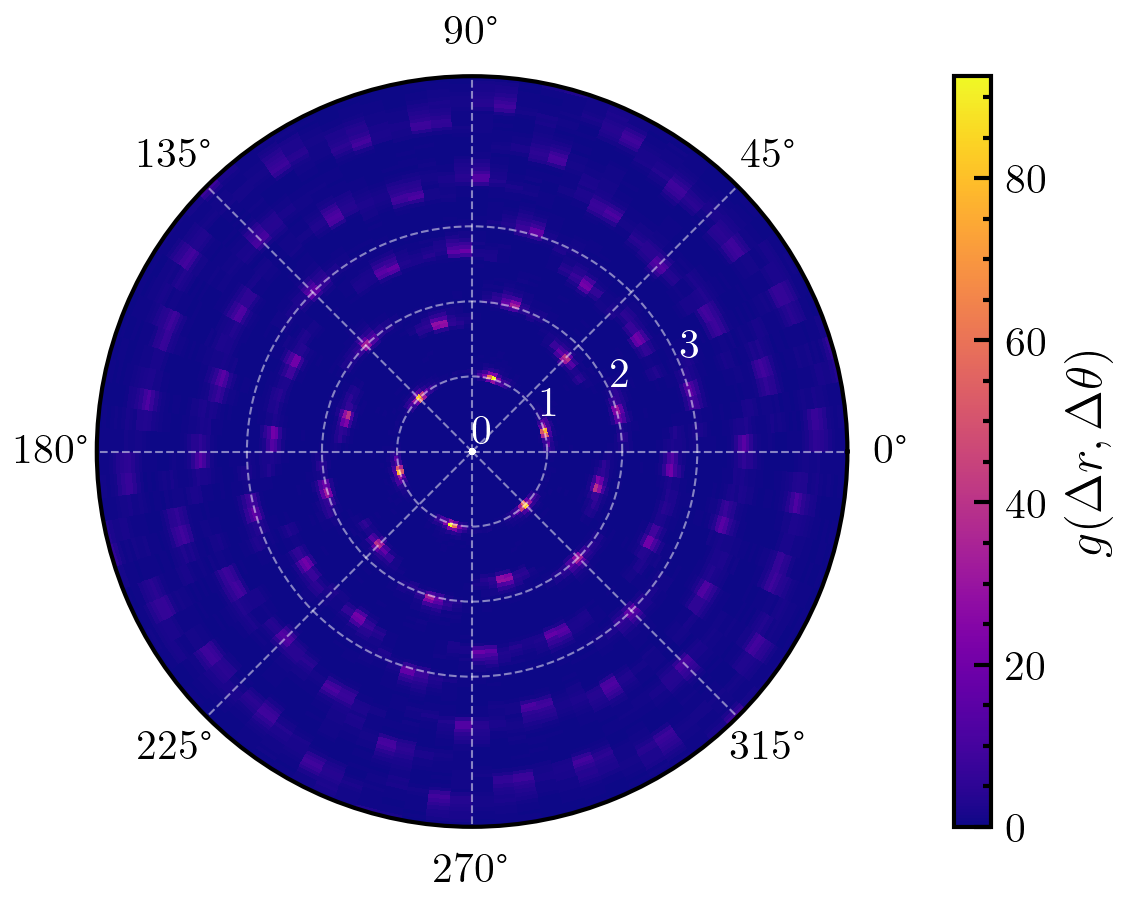
>>> # calculate angular pcf with respect to particle orientations
>>> grt, r, t = amep.spatialcor.pcf_angle(
...        frame.coords(),
...        frame.box,
...        psi = None,
...        e=frame.orientations(),
...        nabins=36,
...        rmax=3,
...        ndbins=100
...    )
>>> fig, axs = amep.plot.new(subplot_kw=dict(projection="polar"))
>>> mp = axs.pcolormesh(t,r, grt)
>>> cax = amep.plot.add_colorbar(fig, axs, mp,
>>>        label=r"$g(\Delta r, \Delta \theta)$")
>>> axs.grid(alpha=.5, lw=.5, c='w')
>>> axs.set_rticks([0,1,2,3])
>>> axs.set_rlim(0,1.1)
>>> axs.tick_params(axis='y', colors='white')
>>> fig.savefig('spatialcor-pcf_angle_2.png')